As I was writing a booklet for an astronomy class I was teaching, I looked for illustrations to explain various elements of celestial mechanics. But I wanted the style of all the illustrations to be coherent. So just fetching images from Wikipedia wasn’t enough.

Since I was writing the booklet with LaTeX, I decided to use TikZ to create my own illustrations. I found a few examples of Solar System illustrations on the excellent texample.net. But I found them a bit autere. I wanted something with more of a cartoon feel, to try to make the booklet more appealing.

Finally, I decided to create all the figures myself with TikZ. I drew little sketches of each planet, the Moon and the Sun that could easily be placed anywhere in a figure. And once I had written the commands to draw these, I created a package that I published on CTAN.

Here are the general ideas for using this package, and a few examples of the possibilities that it offers.

List of examples

• Earth’s equator and the inclination of the Earth
• Lunar phases
• One astronomical unit
• Seasons and Earth’s orbit
• Eclipses (solar and lunar)
• Inclination of the Moon’s orbit
• Conjonctions, oppositions and quadratures
• Lagrange points
• Properties of the planets
• Celestial coordinates

The basics

Let’s start out with a few general ideas on how to use this package. In the document header, add the line

\usepackage{planets}

Then, within a tikzpicture environment, you can draw planets with the command \planet.

\documentclass[varwidth,margin=.3cm]{standalone} 
\usepackage{planets} 
\begin{document} 
\begin{tikzpicture}
\planet[]
\end{tikzpicture}
\end{document}

The \planet command has many options that can be added to make it look like an actual planet of the Solar System. These options can be set in any order.

Setting the aspect of a planet

Surfaces

Specify which celestial body you want to draw with the keyword surface=. The available surfaces are:

• sun
• mercury
• venus
• earth
• moon
• mars
• jupiter
• saturn
• uranus
• neputne
• pluto

For example, you can use \planet[surface=pluto] to draw one of my favorite planetary bodies.

Of course, the Sun, the Moon and Pluto are not planets (but respectively a star, a satellite and a dwarf planet). But they can still be drawn with the same commands as the planets.

Phases

You can also add a phase to your planetary body, if you want to show which part is lit up by the Sun. Do this with the keyword phase=. The available phases are:

• new
• first crescent
• first half
• waxing gibbous
• full
• waning gibbous
• last half
• last crescent
• top
• bottom

For example, you can use \planet[surface=moon, phase=first half] to show the Moon with half of its visible side lit up.

If no phase is specified in the \planet command, then no shadow is drawn.

Rings

You can also add fine rings around a planet by indicating their diameter with the keyword ring=. The unit used to indicate the size of the rings is the diameter of the planet. For instance, \planet[ring=2] will draw rings that are twice as big as the planet.

Saturn has much bigger rings than the other gaseous planets, and is drawn with its rings by default. But you can also add Saturn-like rings to any planet with the option rings. For instance, \planet[surface=earth, rings] will draw an imaginary planet that looks a bit like the Earth but that has huge rings around it.

Planetary rotation

Planets can rotate around an axis. And this axis can be tilted relative to the ecliptic. You can explicitly show a planet’s rotation axis with the option rotation. If you want the planet (and of course its rotation axis) to be tilted, you can use the keyword tilt=.

For instance, you can use \planet[surface=uranus, rotation, tilt=87] to show that the planet Uranus is on its side.

The keyword tilt= modifies the orientation of the surface of the planet, its rings (all the ringed planets we know of have rings that are in the planet’s equatorial plane), and the line that shows the direction of the rotation axis of the planet.

Having a picture with several planets in it

To be able to put several planets in a single image, you need to be able to specify the position of each one of these planets. There are two accepted methods for doing this.

• Specify the point where you want the center of the planet to be with the keyword center=.
• Shift the planet in the x-direction or the y-direction with the keywords centerx= and centery= respectively. If the position of the center of the planet is not specified, then it defaults to (0, 0).

Finally, you can change the size of the planets with the keyword scale=. If no scale is specified, then the default radius for a planet is 1.

---

And that’s it for the basics. Now let’s see some examples of what can be done with this package!

Equator and inclination of the Earth

In astronomy, North and South poles are the two points on the surface of the Earth that the Earth’s rotation axis go through. The equator is the plane that is equidistant between these two points.

The Earth’s rotation axis has a 23.5° inclination compared to the direction orthogonal to the plane that contains the Earth’s orbit.

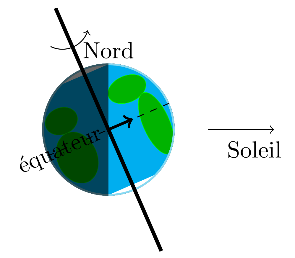
First, draw the Earth (surface=earth) with the rotation axis on (rotation). Tilt the Earth by 23.5° (tilt=23.5). Of course, the Earth is only lit on one side (phase=first half).

\begin{tikzpicture}
    \planet[surface=earth, rotation, tilt=23.5, phase=first half]
	
    \draw [->] (1.5, 0) -- (2.5, 0) ;
    \node (Sun) at (2.2, -.3) {Soleil};
	
    \node at (0, 1.2) {Nord};
    \node[anchor=east, rotate=23.5] at (0, 0) {équateur};
\end{tikzpicture}

Lunar phases

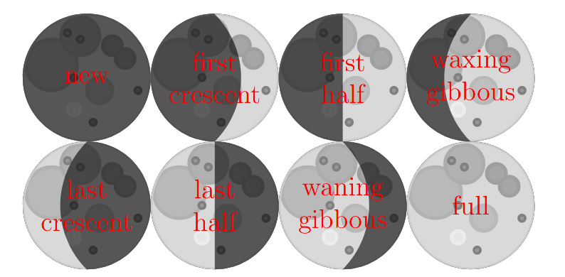
To illustrate the phases of the Moon (and to show all the options available for the keyword phase=), you can draw the eight phases of the Moon. Their position is specified by creating a node with the command \node and setting the planet at that node with the keyword center=(name of the node). This node is also used to set the position of the label indicating the name of that phase.

\begin{tikzpicture}
    \node (new) at (0, 0) {};
    \planet[surface=moon, phase=new, center=(new)]
    \node[red] at (new) {new};

    \node (fc) at (2, 0) {};
    \planet[surface=moon, phase=first crescent, center=(fc)]
    \node[red, align=center] at (fc) {first \\ crescent};

    \node (fh) at (4, 0) {};
    \planet[surface=moon, phase=first half, center=(fh)]
    \node[red, align=center] at (fh) {first \\ half};

    \node (wxg) at (6, 0) {};
    \planet[surface=moon, phase=waxing gibbous, center=(wxg)]
    \node[red, align=center] at (wxg) {waxing \\ gibbous};

    \node (full) at (6, -2) {};
    \planet[surface=moon, phase=full, center=(full)]
    \node[red, align=center] at (full) {full};

    \node (wng) at (4, -2) {};
    \planet[surface=moon, phase=waning gibbous, center=(wng)]
    \node[red, align=center] at (wng) {waning \\ gibbous};

    \node (lh) at (2, -2) {};
    \planet[surface=moon, phase=last half, center=(lh)]
    \node[red, align=center] at (lh) {last \\ half};

    \node (lc) at (0, -2) {};
    \planet[surface=moon, phase=last crescent, center=(lc)]
    \node[red, align=center] at (lc) {last \\ crescent};
\end{tikzpicture}

One astronomical unit

An astronomical unit is equal to the average Earth-Sun distance. Or more mathematically, to the major axis of the ellipse on which the Earth orbits. This is equal to 149 million kilometers, or 8 light-minutes.

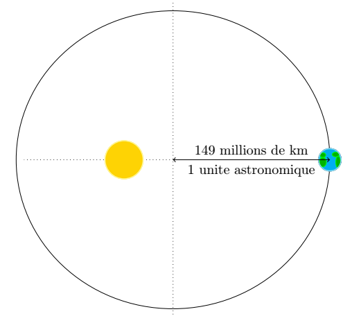
The orbit of the Earth is an ellipse centered in (0, 0) with a major axis equal to \a and a minor axis equal to \b. The Sun is located at a focus of this ellipse in (0, \f). The location of the Sun is computed given the major and minor axes of the ellipse.

\begin{tikzpicture}
\def\a{4} % demi-grand axe
    \def\b{3.8} % demi-petit axe
    \def\f{{-sqrt(\a*\a-\b*\b)}} % position du foyer de l'ellipse

    % Orbite de la Terre
    \draw (0,0) ellipse ({\a} and {\b});

    % Axes de l'ellipse
    \draw[dotted] (0, \a) -- (0, -\a);
    \draw[dotted] (\b, 0) -- (-\b, 0);

    % Soleil
    \planet[surface=sun, centerx=\f, scale=.5]

    % Terre
    \planet[surface=earth, centerx=\a, scale=.3]

    % Unité astronomique
    \draw[<->] ({\a}, 0) -- node[below] {1 unite astronomique} node[above] {149 millions de km} (0, 0) ;
\end{tikzpicture}

Seasons and the Earth’s orbit

Seasons on Earth are caused by the inclination of the Earth’s rotation axis and the motion of the Earth around the Sun. This is why it is winter in the Northern hemisphere when it is summer in the Southern hemisphere, and vice versa.

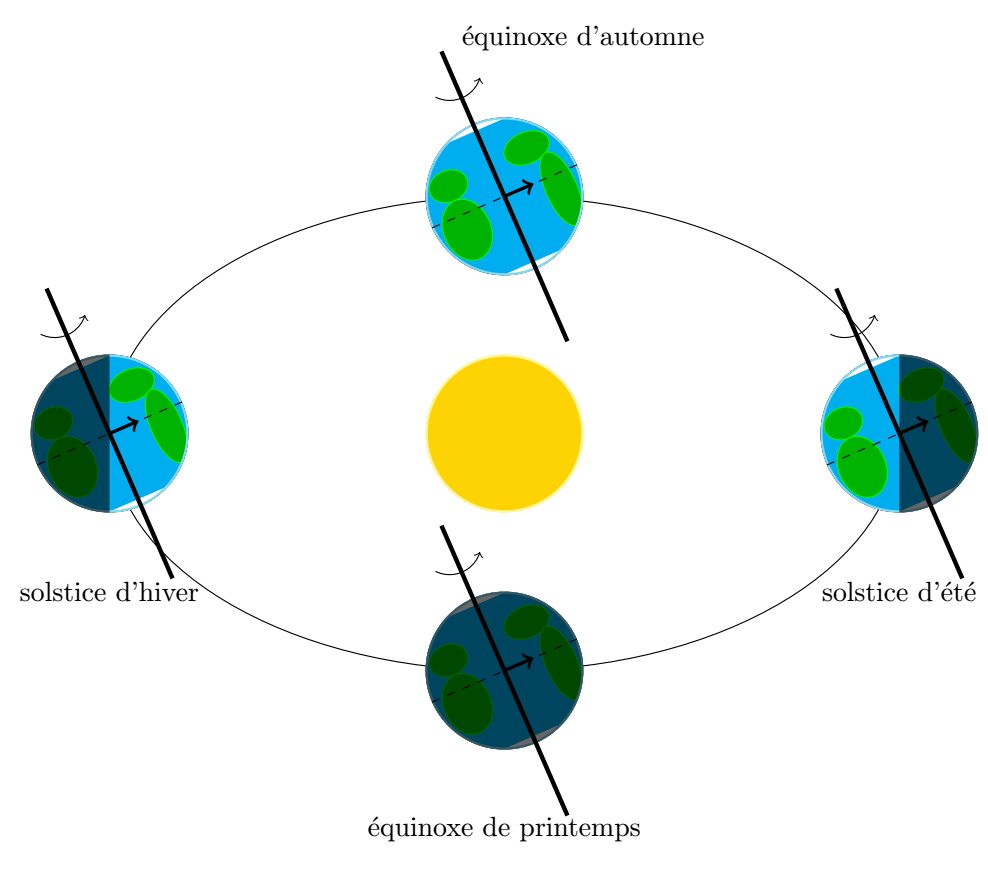
Draw the Sun in the center, and the Earth in four different positions with four different phases. The tilt of the Earth’s rotation axis is constant over time tilt=23.5.

\begin{tikzpicture}
    \planet[surface=sun]
    \draw (0, 0) circle (5 and 3);

    \planet[surface=earth, phase=first half, rotation, tilt=23.5, centerx=-5]
    \node at (-5, -2) {solstice dhiver};

    \planet[surface=earth, phase=last half, rotation, tilt=23.5, centerx=5]
    \node at (5, -2) {solstice dété};

    \planet[surface=earth, phase=new, rotation, tilt=23.5, centery=-3]
    \node at (0, -5) {équinoxe de printemps};

    \planet[surface=earth, phase=full, rotation, tilt=23.5, centery=3]
    \node at (1, 5) {équinoxe dautomne};
\end{tikzpicture}

Eclipses (solar and lunar)

When the Moon passes directly between the Earth and the Sun, a solar eclipse happens.

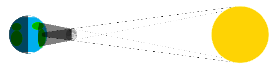
Getting all the line properly set up in this picture is a bit more difficult. I had to do some computations on a piece of paper to get all the lines to intersect right where they should.

\begin{tikzpicture}
    \draw[dashed] (-3, 0) -- (8, 1.5);
    \draw[dashed] (-3, 0) -- (8, -1.5);

    \draw[dotted] (-3, -0.76) -- (8, 1.5);
    \draw[dotted] (-3, 0.76) -- (8, -1.5);

    % Les trois astres
    \planet[surface=moon, scale=.3, centerx=-.75]
    \planet[surface=sun, centerx=8, scale=1.5]
    \planet[surface=earth, centerx = -3, phase=first half]

    % Ombre
    \begin{scope} 
        \clip[overlay] (-.1, 0) circle (2.2);
        \fill[opacity=.5] (-.75, .3) -- (-3, 0) -- (-.75, -.3) -- cycle;
    \end{scope}

    % Pénombre
    \begin{scope}
        \clip[overlay] (0, 0) circle (2.5);
        \fill[opacity=.5] (-.75, .3) -- (-3, .75) -- (-3, -.75) -- (-.75, -.3) -- cycle;
    \end{scope}
\end{tikzpicture}

And when the Moon goes through the shadow of the Earth, that’s a lunar eclipse.

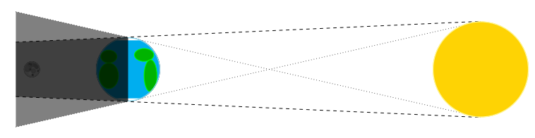
\begin{tikzpicture}
    \draw[dashed] (-3.5, .85) -- (11, 1.5);
    \draw[dashed] (-3.5, -.85) -- (11, -1.5);

    \draw[dotted] (-3.5, -1.8) -- (11, 1.5);
    \draw[dotted] (-3.5, 1.8) -- (11, -1.5);

    \planet[surface=moon, scale=.25, centerx=-3]
    \planet[surface=sun, centerx=11, scale=1.5]
    \planet[surface=earth, centerx = 0]

    \fill[opacity=.5, black] (0, 1) -- (-3.5, .85) -- (-3.5, -.85) -- (0, -1) -- cycle;
    \fill[opacity=.5, black] (0, 1) -- (-3.5, 1.8) -- (-3.5, -1.8) -- (0, -1) -- cycle;
\end{tikzpicture}

Inclination of the orbit of the Moon

The Moon doesn’t orbit in exactly the same plane as the Earth does. This is why eclipses don’t happen every month.

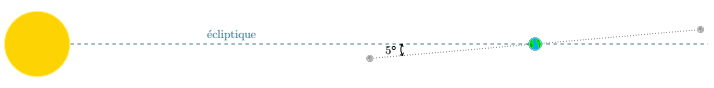
For this picture, I cheated a bit. The Moon’s orbit is only tilted by 5° compared to the ecliptic, but to make the sketch easier to understand, I tilted it by 10°.

\begin{tikzpicture}
    \draw[dashed, color=cyan!50!black] (-10, 0) --  (2, 0);
    \node[above right, color=cyan!50!black] at (-8, 0) {écliptique};

    \draw[dotted] (190:2.5) -- (10:2.5);

    \planet[surface=sun, centerx=-10]

    \planet[surface=earth, scale=.2]

    \planet[surface=moon, scale=.1, centerx=-2, centery=-.4]
    \planet[surface=moon, scale=.1, centerx=2, centery=.4]

    \draw [<->] (180:2.2) to [bend right=30]  node [left] {5$^\circ$} (190:2.2);
\end{tikzpicture}

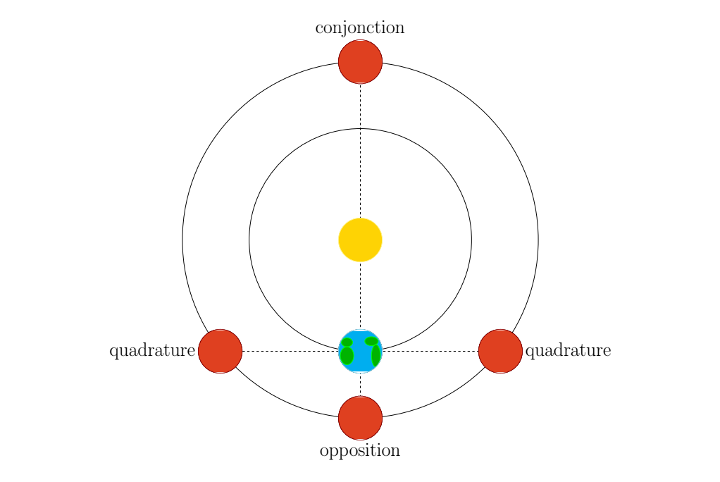
Conjonctions, oppositions and quadratures

For an outer planet (Mars to Neptune), a conjunction is when the planet is behind the Sun relative to the Earth. An opposition is when the planet is its closest to us (so on the opposite end of the sky compared to the Sun, hence the name). And a quadrature is when the Sun, the Earth and the outer planet form a 90° angle.

\begin{tikzpicture}
    \draw[dashed] (-5.3, 0) -- (5.3, 0);
    \draw[dashed] (0, 13) -- (0, -3);
    
    \draw (0, 5) circle (5);
    \planet[surface=earth]
    \planet[surface=sun, centery=5]
    
    \draw (0, 5) circle (8);    
    \planet[surface=mars, centery=-3]
    \node[below] at (0, -4) {\Huge opposition};
    
    \planet[surface=mars, centery=13]
    \node[above] at (0, 14) {\Huge conjonction};
    
    \planet[surface=mars, centerx=6.3]
    \node[right] at (7.3, 0) {\Huge quadrature};
    
    \planet[surface=mars, centerx=-6.3]
    \node[left] at (-7.3, 0) {\Huge quadrature};
\end{tikzpicture}

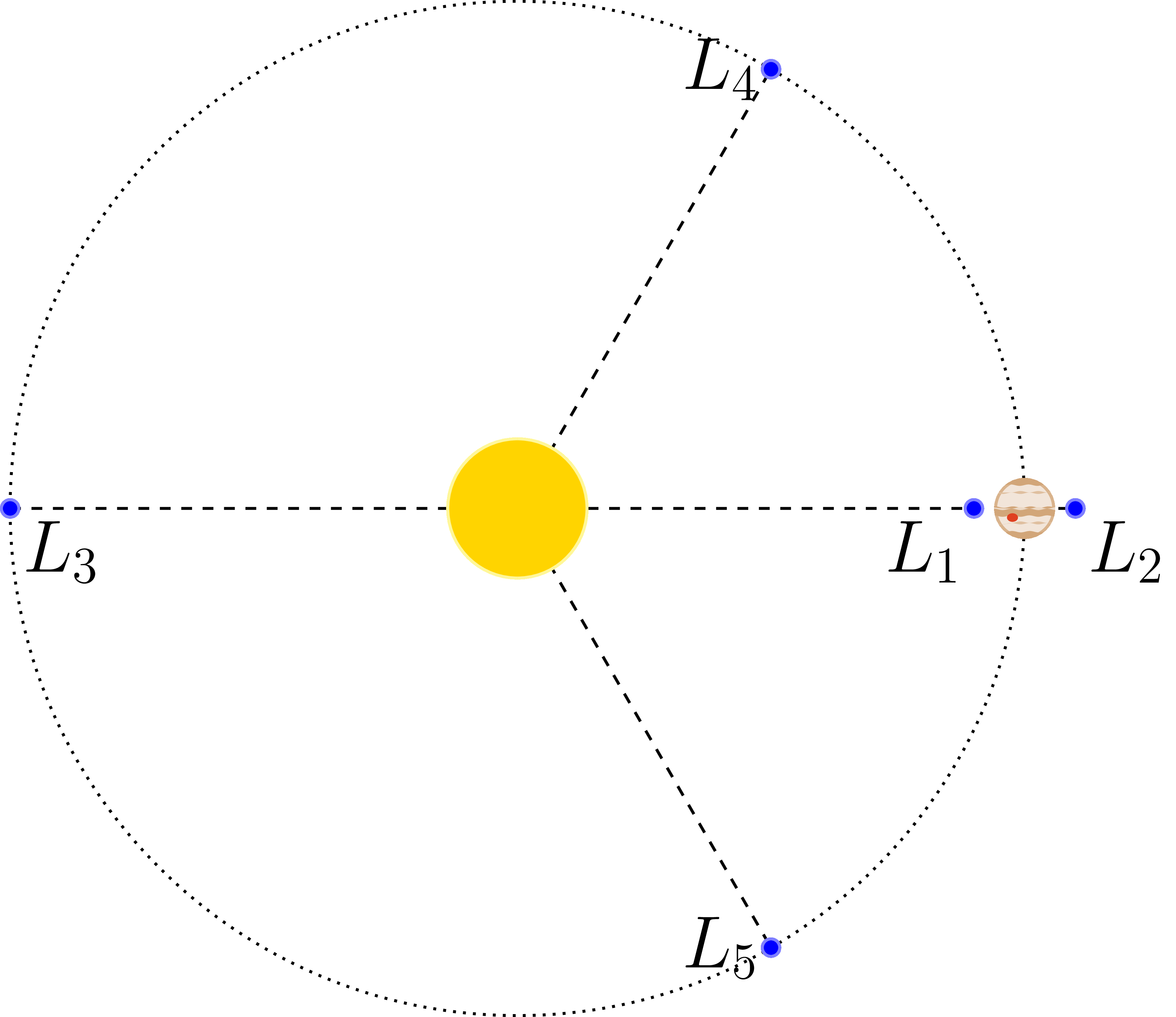
Lagrange points

In the 3-body problem, there are certain stable configurations. These are called Lagrange points.

\begin{tikzpicture}
\draw [thick, dashed] (-5, 0) -- (5.5, 0);
\draw [thick, dashed] (0, 0) -- (60:5);
\draw [thick, dashed] (0, 0) -- (-60:5);

\draw [thick, dotted] (0, 0) circle (5);
\planet[surface=sun, scale=.7]
\planet[surface=jupiter, center={(5, 0)}, scale=.3]

\planet[color=blue, scale=.1, center={(60:5)}]
\node [left] at (60:5) {\huge $L_4$};

\planet[color=blue, scale=.1, center={(-60:5)}]
\node [left] at (-60:5) {\huge $L_5$};

\planet[color=blue, scale=.1, center={(4.5, 0)}]
\node [below left] at (4.5, 0) {\huge $L_1$};

\planet[color=blue, scale=.1, center={(5.5, 0)}]
\node [below right] at (5.5, 0) {\huge $L_2$};

\planet[color=blue, scale=.1, center={(-5, 0)}]
\node [below right] at (-5, 0) {\huge $L_3$};
\end{tikzpicture}

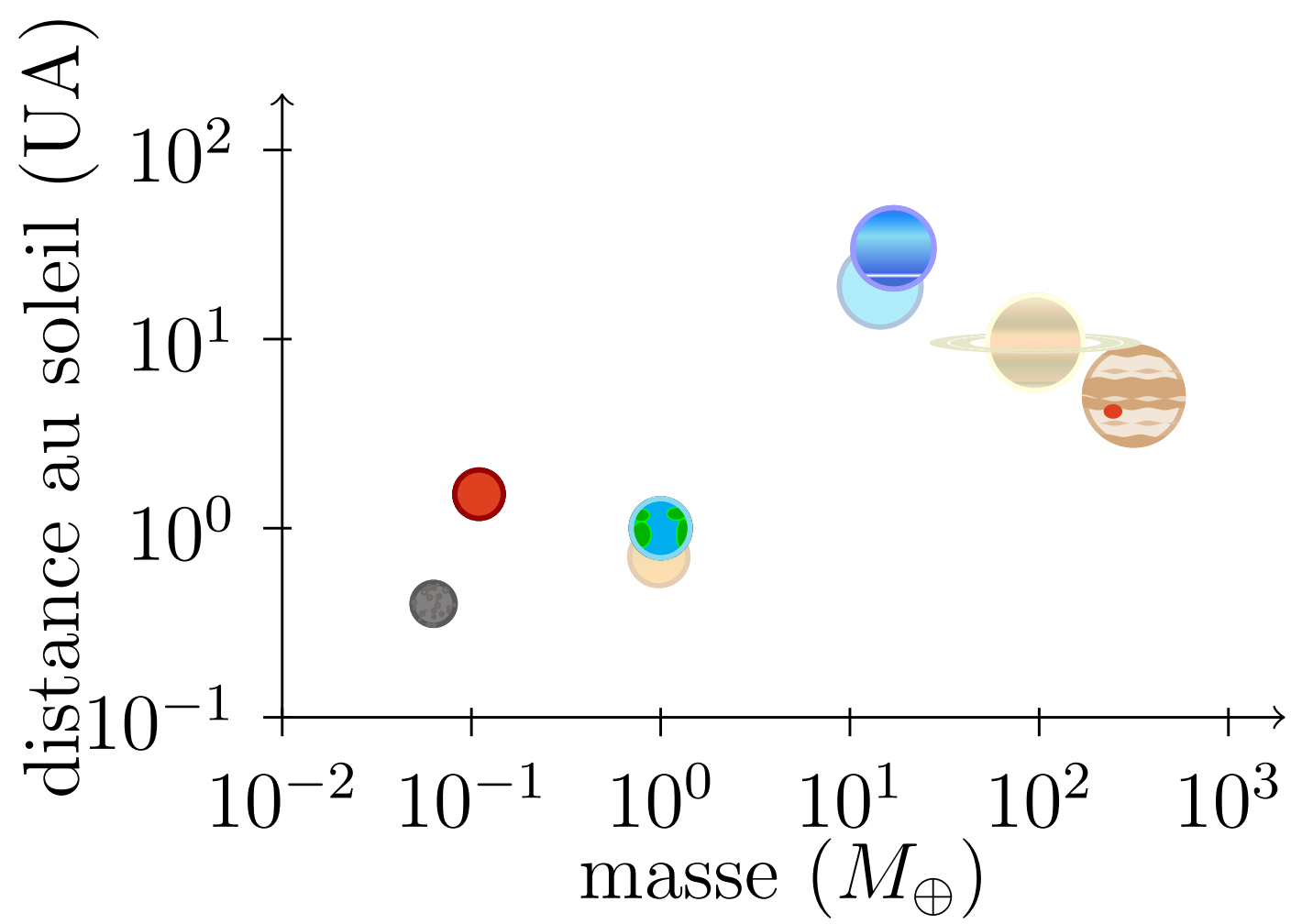
Properties of the planets

The planets of our solar system can by sorted based on their mass, their diameter and the diameter of their orbit.

\begin{tikzpicture}

% On défini d'abord quelques macros pour faciliter la création des axes du graphique
\pgfmathsetmacro{\xorigin}{-2}
\pgfmathsetmacro{\yorigin}{-1}
\pgfmathsetmacro{\xend}{3.3}
\pgfmathsetmacro{\yend}{2.3}
\pgfmathsetmacro{\xtwo}{-1}
\pgfmathsetmacro{\ytwo}{0}
\pgfmathsetmacro{\ticksize}{0.1}

\coordinate (origin) at (\xorigin, \yorigin);
\coordinate (absend) at (\xend, \yorigin);
\coordinate (ordend) at (\xorigin, \yend);

% Puis on trace les axes...
\draw [->] (origin) -- coordinate (xmid) (absend);
\draw [->] (origin) -- coordinate (ymid) (ordend);

% ... avec leurs graduations
\foreach \x in {\xorigin, \xtwo,...,\xend}
	\draw (\x, \yorigin + 0.5*\ticksize) -- (\x, \yorigin - \ticksize)
	node[anchor=north] {$10^{\pgfmathprintnumber\x}$};
\foreach \y in {\yorigin, \ytwo,...,\yend}
	\draw (\xorigin + 0.5*\ticksize, \y) -- (\xorigin - \ticksize, \y)
	node [anchor=east]{$10^{\pgfmathprintnumber\y}$};

% On place la légende des axes
\node[below = 1.2em] at (xmid) {masse ($M_\oplus$)}; %xaxis
\node[rotate = 90, above = 2em] at (ymid) {distance au soleil (UA)}; %yaxis

% Enfin, on place les planètes au bon endroit, avec le diamètre qui est fonction du diamètre réel
\planet[surface=mercury, center={(-1.2, -0.4)}, scale=0.128]
\planet[surface=venus, center={(-.01, -.15)}, scale=0.168]
\planet[surface=earth, center={(0, 0)}, scale=0.170]
\planet[surface=mars, center={(-0.96, 0.18)}, scale=0.142]
\planet[surface=jupiter, center={(2.5, 0.7)}, scale=0.275]
\planet[surface=saturn, center={(1.98, 0.98)}, scale=0.267]
\planet[surface=uranus, center={(1.16, 1.28)}, scale=0.230]
\planet[surface=neptune, center={(1.23, 1.48)}, scale=0.229]

\end{tikzpicture}

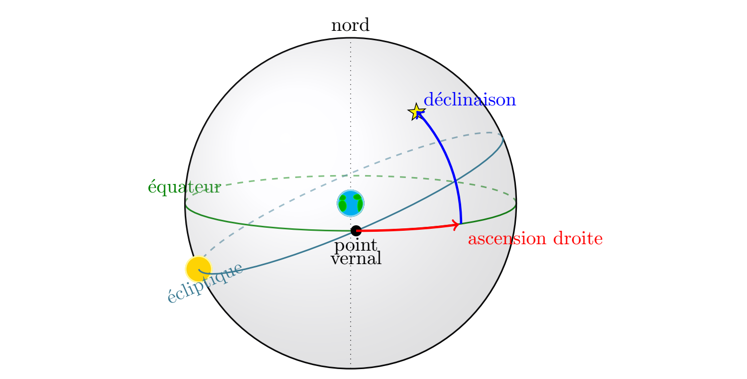
Celestial coordinates

As a last example, here is the code that was used to make the drawing in the header of this article.

To draw a star, you have to import an extra TikZ library by adding the command \usetikzlibrary{shapes} to the header

\begin{tikzpicture}%
\node (dec) at (1.2, 1.65) {};
\node (ad) at (2, -.375) {};

% Axe nord-sud
\draw[dotted] (0, -3) -- (0, 3);
\node[above] at (0, 3) {nord};

% Équateur
\draw[thick, color=green!50!black] (-3,0) arc (180:360:3 and .5);
\draw[thick, dashed, opacity=.6, color=green!50!black] (-3,0) arc (180:0:3 and .5);
\node[color=green!50!black, above] at (-3, 0) {équateur};

% Écliptique (arrière)
\draw[thick, dashed, rotate=23.5, color=cyan!50!black, opacity=.6] (-3,0) arc (180:0:3 and .5);
% Celestial sphere
\draw[thick] (0,0) circle (3);
\shade[ball color=blue!5!white,opacity=0.20] (0,0) circle (3);

% Terre
\planet[surface=earth, scale=.25]
% Soleil
\planet[surface=sun, scale=.25, centerx = -2.751, centery = -1.196]

% Ecliptique (avant)
\draw[thick, rotate=23.5, color=cyan!50!black] (-3,0) arc (180:360:3 and .5);
\node[color=cyan!50!black, rotate=24, below] at (203.5:3) {écliptique};

% Point vernal
\node (gamma) at (0.1,-.5)  {};
\node[below, align=center] at (gamma) {point \\[-.5em] vernal};
\fill(gamma) circle (.1);

% Étoile
\node[star,star points=5, draw, fill=yellow, star point ratio=0.4, rotate=40] (star) at (dec) {};

% Ascension droite
\draw[red, very thick, ->] (gamma) arc (-90:-50:2.9 and .5);
\node[below right, red] at (ad) {ascension droite};

% Déclinaison
\draw[blue, very thick, ->] ++(ad) arc (0:43:3);
\node [blue, above right] at (dec) {déclinaison};
\end{tikzpicture}

Conclusion

Here are a few examples of what you can do with TikZ-planets. I hope this article gave you some inspiration for your own illustrations.